CS229 Linear Regression - Flash's Ideal

INFO
This is my study note of the Stanford CS229 (Spring 2018), based on my understanding and the course notes released on the official website.

The note focuses on important ideas and formulas in machine learning, ignoring overt definitions and long derivations.

LMS algorithm#

We now know that the cost function is $J(\theta)=\frac{1}{2}\sum_{i=1}^{m}(h_{\theta}(x^{(i)})-y^{(i)})^2$ , then let’s consider the gradient descent algorithm to minimize $J(\theta)$ .

\theta_j:=\theta_j-\alpha\dfrac{\partial}{\partial \theta_j}J(\theta)

Here, $\alpha$ is called the learning rate.

And we have $\dfrac{\partial}{\partial \theta_j}J(\theta)=(h_{\theta}(x)-y)x_j$ , then

\theta_j:=\theta_j+\alpha\left(y^{(i)} - h_{\theta}(x^{(i)})x^{(i)}_j \right)

The rule is called the LMS (least mean squares) update rule and is also known as the Widow-Hoff learning rule.

Our first algorithm using LMS rule is batch gradient descent, it’s main process is as follows:

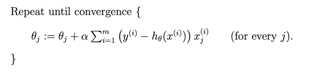
For every $\theta_j$ , we have to run over the entire training set. Note that gradient descent algorithm can be susceptible to local minima in general.

Consider another algorithm called stochastic (incremental) gradient descent, it is as follows:

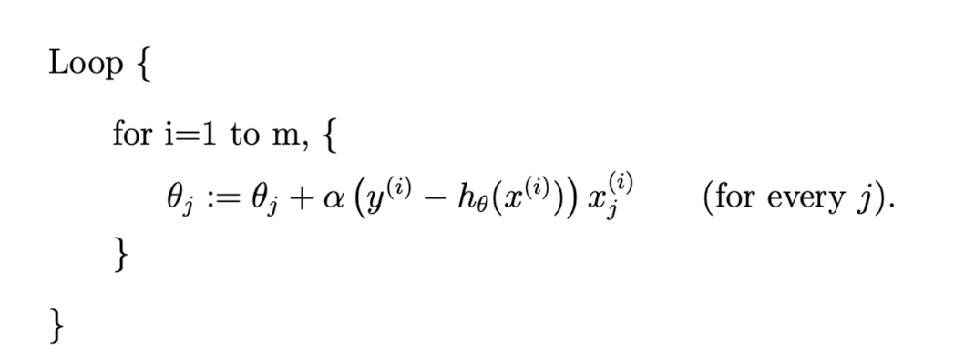
In this algorithm, the $\theta$ is updated every time we encounter a training example.

Compare with batch gradient descent, stochastic gradient descent has several advantages:

While batch gradient descent has to scan over the whole set to update a single $\theta_j$ , stochastic gradient descent can start making progress right away.
It gets $\theta$ close to the minimum much faster. (Note that it can never “converge” to the minimum)

For these reasons, we prefer stochastic gradient descent when the training set is large.

The normal equations#

The second way of minimizing $J$ is to do calculus with matrices.

Matrix derivatives#

We define the derivative of $f: \mathbb{R}^{m\times n}\mapsto\mathbb{R}$ with respect to $A$ to be:

\nabla_A f(A)=\begin{bmatrix} \frac{\partial f}{\partial A_{11}} & \cdots & \frac{\partial f}{\partial A_{1n}} \\ \vdots & \ddots & \vdots \\ \frac{\partial f}{\partial A_{n1}} & \cdots & \frac{\partial f}{\partial A_{nn}} \end{bmatrix}

For trace operator, we have:

\mathrm{tr}A=\mathrm{A^T} \\ \mathrm{tr}(A+B)=\mathrm{A}+\mathrm{B} \\ \mathrm{tr}aA=a\mathrm{tr}A$$ For combinations of these two operations, we have:

\nabla_A \mathrm{tr}AB=B^T \ \nabla_{A^T} f(A) = (\nabla_A f(A))^T \ \nabla_A \mathrm{tr}ABA^TC=CAB + C^T AB^T \ \nabla_A|A| = |A|(A^{-1})^T

### Least squares revisited The training set's input can be written as the following matrix:

X = \begin{bmatrix} - (x^{(1)})^T - \ - (x^{(2)})^T - \ \vdots \ - (x^{(m)})^T - \end{bmatrix}

Also, let $\vec{y}$ be

\vec{y}=\begin{bmatrix} y^{(1)} \ y^{(2)} \ \vdots \ y^{(m)} \end{bmatrix}

Now, since $h_{\theta}(x^{(i)}) = (x^{(i)})^T\theta$, we can verify that:

J(\theta) = \frac{1}{2}(X\theta-\vec{y})^T(X\theta-\vec{y})

To minimize $J$, we can derive that:

\partial_{\theta}J(\theta)=X^TX\theta - X^T\vec{y}

Then we obtain the **normal equations**:

X^TX\theta = X^T\vec{y}

Thus, the value of $\theta$ that minimizes $J$ is:

\theta = (X^TX)^{-1}X^T\vec{y}

## Probabilistic interpretation To discover whether $J$ is a reasonable choice, let us assume that the target variables and the inputs are related via the equation

y^{(i)} = \theta^T x^{(i)} + \epsilon^{(i)}

Let us further assume that the $\epsilon^{(i)}$ are distributed IID (independently and identically distributed) according to a Gaussian distribution. We can write this as following:

p(y^{(i)}|x^{(i)};\theta)=\dfrac{1}{\sqrt{2\pi}\sigma}\exp\left(-\dfrac{(y^{(i)} - \theta^Tx^{(i)})^2}{2\sigma^2}\right)

To view this as a function of $\theta$, we instead call it the **likelihood** function:

\begin{aligned} L(\theta) &= L(\theta;X,\vec{y})=p(\vec{y}|X;\theta) \ &= \prod_{i=1}^m p(y^{(i)}|x^{(i)};\theta) \end{aligned}

The principal of **maximum likelihood** says we should choose $\theta$ to maximize $L(\theta)$. To make it simpler, we instead maximize the **log likelihood** $\ell(\theta)$:

\begin{aligned} \ell(\theta) &= \log L(\theta) \ &= m\log\frac{1}{\sqrt{2\pi}\sigma}-\frac{1}{\sigma^2}\cdot\frac{1}{2}\sum_{i=1}^{m}(y^{(i)} - \theta^T x^{(i)})^2 \end{aligned}

Hence, maximizing $\ell$ is the same as minimizing $\frac{1}{2}\sum_{i=1}^m(y^{(i)}-\theta^Tx^{(i)})^2=J(\theta)$. Note that our final choice of $\theta$ did not depend on $\sigma^2$. ## Locally weighted linear regression In contrast to the original linear regression algorithm, the locally weighted regression gives every $\epsilon^{(i)}$ a weight $w^{(i)}$, thus we can "ignore" some bad training examples. A fair standard choice for the weights is:

w^{(i)}=\exp\left(-\dfrac{(x^{(i)} - x)^2}{2\tau^2}\right)

As a **non-parametric** algorithm, to make predictions using locally weighted linear regressions, we need to keep the entire training set around for $h$ to grow linearly with the size of the training set.